In this article we will explore one of the most challenging tools to use in a mix: the compressor. A compressor can be incredibly rewarding, but it can also cause plenty of headaches, and using it correctly is one of the clearest signs of a seasoned professional. Everyone has their own philosophy when it comes to compression, and the amount of compression we apply—as well as the settings we choose—depends heavily on the musical material we are working with.

In this installment, we’ll try to learn how to use a compressor properly by studying how these devices work and reviewing practical examples. We will also analyze the role a compressor plays within a mix and discuss the different types of compressors that exist.

Dangerous Curves

As more and more tracks have been added to modern music productions, more and more compressors have also been introduced. Today, the sound of contemporary productions is heavily characterized by the use of numerous compressors. However—as we all know—modern music is not exactly known for having great dynamic range. Many people tend to overcompress everything that passes through their hands. We must remember that one of the most important characteristics of music is precisely its dynamics, and dynamics are largely what prevent a song from becoming boring. If a piece of music has changes in intensity, it will keep the listener engaged, while a completely flat, linear song will bore even the members of the band itself.

It is therefore crucial that we preserve the natural dynamics of the song we are mixing. For example, imagine a rock track where halfway through the arrangement the drums drop out and only acoustic guitars and a vocal remain. That section should clearly sound quieter than the rest of the track. Today, unfortunately, it’s not uncommon to hear songs with an intro without drums that plays at exactly the same loudness as the rest of the track. This completely destroys the artistic intention the musicians had—most likely they wanted the entrance of the drums to feel like a lift or impact for the listener. Another clear example of today’s overcompression is found in mixes where the vocal maintains exactly the same loudness from the very beginning to the very end. This often happens because of improper compression or limiting on vocal tracks. It completely ruins the artistic sense of the song by making its most important element dull and lifeless. Haven’t you ever had a teacher in high school or university who spoke at the exact same volume from the beginning to the end of class? Personally, I had several—and ten minutes into the lesson I was already nodding off.

Beyond that, we must also consider the natural dynamics that each instrument has within the musical piece and try to preserve that as well. Many people say that modern genres like rock or metal have no dynamics whatsoever. Well, that is partly true, but not entirely. It’s true that these styles don’t lend themselves to big dynamic contrasts between sections, but they do rely on a very powerful rhythmic foundation. Today, however, people tend to over-flatten that rhythmic foundation, which results in the kick/snare interplay becoming unexciting and failing to make us tap our foot (or headbang, in the case of metalheads).

Many so-called professionals place the blame for overcompression on mastering engineers. However, in many cases the mixing engineer is more responsible than the mastering engineer. Now imagine what happens when you combine a bad mixing engineer with a bad mastering engineer—the results can be disastrous, reaching truly absurd levels of overcompression.

An overcompressed album with extremely high loudness levels will give us the impression that it sounds better than another that retains its dynamic range, but only if we make a quick A/B comparison—and only for a few seconds. After that, we realize that the music lacks artistic meaning. This is because anything that is louder than something else will initially sound “better.” The reason for this has been widely studied in psychoacoustics and is due to the fact that the human auditory system does not have a linear response—in other words, it does not perceive all frequencies equally.

Munson–Fletcher equal-loudness curves

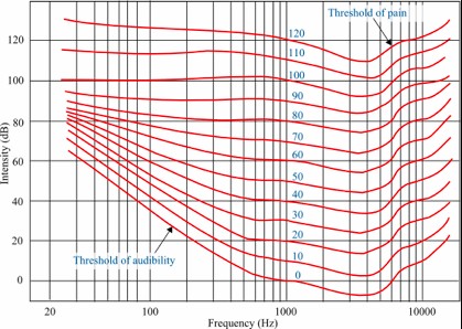
This phenomenon is explained by the equal-loudness curves. The reference point is the perceived loudness produced by a given level at 1 kHz, where human hearing is most sensitive. From there, we determine how many dB SPL (sound pressure level) are needed at all other frequencies to produce the same perceived loudness. This is measured in phons. For example, if we take 0 dB at 1 kHz—which is just above the threshold of hearing—we see that while a 1 kHz tone at 0 dB SPL represents the hearing threshold, at 100 Hz we would need more than 35 dB SPL to begin hearing it. Therefore, at low and high frequencies we need much more level to achieve the same loudness we perceive at mid frequencies. Additionally, we observe that as overall levels rise, the equal-loudness curves flatten, meaning that the required differences at low and high frequencies to match mid-frequency loudness become smaller as playback volume increases.

Now let’s reason through this to see why understanding it is important. Imagine we play our favorite album on our music system at a low volume. Since we need much more level at low and high frequencies to perceive them as loud, we probably won’t hear them at all, perceiving mainly the midrange. Now imagine we suddenly turn up the volume. We will notice that the same record, on the same system, sounds much better. That’s simply because at the higher playback level we can now clearly hear the lows and highs.

Now, if we take into account that equal-loudness curves flatten as playback levels increase, consider the following: imagine that two poor professionals (mixing engineer and mastering engineer) work on a production and the result is an extremely overcompressed album. If we play that album quietly on our system and then immediately play our favorite album—with the system volume unchanged—our favorite record will sound much worse than the overcompressed one, because in this case we are not hearing the lows and highs, even though we know that the second album sounds infinitely better. What is the solution? Easy—pick up the remote control and raise the volume. This way we will enjoy the low and high frequencies on a record with proper dynamics.

We must remember that “non-freak” listeners do not spend time A/B-ing different albums. They get into their car, or sit down in their living room, or turn on their iPod, and simply raise the volume to whatever level feels comfortable, without considering whether one record initially sounds quieter than another. The difference is that with a dynamic record, that listener will enjoy the music—and with an overcompressed one, it’s unlikely they’ll make it past the third track.

The only situation in which we cannot avoid overcompression is when a song is intended for broadcast on radio or television. In that case, due to the technical requirements of those media, we need to push compression further (both in mixing and mastering). But, as with most things in life—except death—there is a simple solution: create special mixes and masters for that purpose. Imagine a band brings you a 12-track album to mix and tells you which three songs will be released as singles. Your job would consist of mixing the 12 album tracks plus a special version of each of the three singles. These are called “radio edits.” These mixes usually feature heavier compression and slightly louder vocals than the “normal” album mixes. We deliver the 12 regular tracks plus the three radio edits to the mastering engineer, indicating the specific purpose of the latter.

As you can see, the so-called “loudness war” is a bit ridiculous, since the solution is quite simple. Fortunately, more and more musicians today are becoming aware of these issues and increasingly request that the natural dynamics of their songs be respected. However, many supposed professionals use all this as an excuse to make their work seem more impressive or impactful than it actually is.

It is therefore essential that whenever we compare two songs, they both have the same loudness level so we can make a truly objective comparison. To do this, we simply check the RMS level of both songs and reduce the volume of the louder one by the number of RMS dB it exceeds the other.

It is also important—especially if you are new to mixing—to remember that when comparing your mixes to commercial tracks you like, those commercial tracks have already been mastered and therefore will have a higher perceived loudness than your unmastered mix, which can easily mislead you for all the reasons explained above.

Types of Compressors

Throughout history, different compression circuits have been developed. Unlike what happens in the “real world,” technological progress has not made older models obsolete or less valuable. Quite the opposite—for example, a Fairchild 660 from the 1960s can easily cost around €25,000 today. The most notable differences between compressor types relate to their gain-control stage. In other words, what defines a compressor is the way in which gain reduction is applied to the incoming signal. Each design philosophy leads to a different sonic character, which is why **each type of compressor sounds distinct**. So even though all compressors perform the same basic task (reducing dynamic range), it is essential to know the characteristic sound of each type and understand how they behave.

If we look at the circuits that determine gain reduction in compressors, we can classify them as follows:

• Variable-mu. These were the first compressors ever implemented. Their operation is based on a special type of tube called a variable-mu tube. Its key characteristic is the ability to dynamically change gain as a function of the input signal level. Because of this, variable-mu compressors typically do not have a ratio control—the amount of gain reduction is directly dependent on the input level. The Fairchild 660 and its stereo version, the 670, as well as the Manley Variable Mu, are classic examples of this type.
• FET. When semiconductors entered the world of electronics, they often replaced large vacuum tubes with much smaller components known as transistors. This type of compressor is based on a special transistor called a field-effect transistor (FET). These compressors have a very clean, bright sound and generally feature fast attack and release times. Additionally, FET compressors handle large amounts of gain reduction much more gracefully than other types. They also introduced a now-familiar control: the ratio—although rather than offering a continuous ratio control, only a few fixed settings can be selected. The classic example in this category is the UREI 1176LN.
• Optical. The gain-reduction stage in optical compressors is based on a light-dependent system. On one side, a light source (incandescent or LED) responds to variations in input level—the higher the level, the brighter the light. On the other side, a photosensitive component (typically a phototransistor) reacts to these light changes, reducing gain accordingly. Because of the nature of the light circuit, these compressors tend to have slow attack and release times—they are generally very “slow” compressors. They have a very distinctive sound, which is why they continue to be widely used today. Classic examples include the Teletronix LA-2A and the UREI LA-3A. The main difference is that the LA-2A uses a tube-based amplification stage, while the LA-3A uses transistors.
• VCA. These are the “standard” compressors we are most accustomed to using. They are the go-to devices for controlling the dynamics of individual tracks when a specific coloration or character is not desired. These solid-state (transistor-based) compressors allow very precise control of gain reduction thanks to their fast response and highly consistent transfer curves.

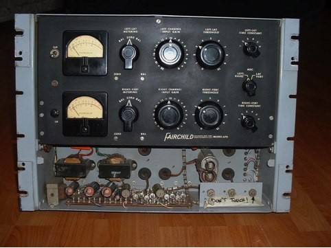
Fairchild 670 — Variable-mu compressor

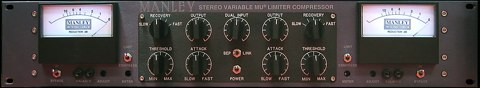
Manley Variable Mu — Variable-mu compressor

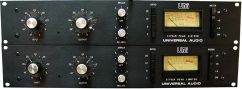
Stereo pair of UREI 1176LN compressors — FET compressors

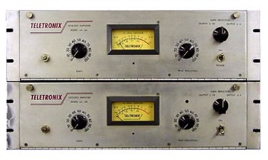
Stereo pair of Teletronix LA-2A compressors — Optical compressors

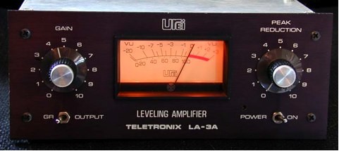
Urei LA-2A — Optical compressor

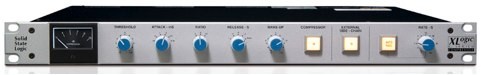
SSL XLogic G Series stereo compressor — VCA compressor

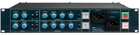
Neve 33609U stereo compressor — VCA compressor

Why Use Compressors?

As audio production technology has advanced, we’ve gained the ability to use more and more tracks in a session. Today, thanks to computer-based digital systems, we practically have no limits on track count. It’s common to find mixes with 70 tracks or more, each with its own natural dynamics.

The first reason to use compressors is to keep the dynamics of all the tracks in a mix under control. Everyone has their own philosophy, but I usually compress almost every track—very subtly. I like my mixes to have a cohesive, compact sound, and that requires taming unruly peaks. This philosophy can be dangerous, though, because if we overdo it, we can easily suck the life out of the sound. Usually, just 2 or 3 dB of gain reduction is more than enough for this purpose. We must also consider the musical style. Some genres—like jazz or classical music—rarely use compression. In these cases, the expectation is that the sound remains as natural as possible, so compressors should be avoided unless absolutely necessary on a specific track.

Another reason to use compressors is to level out signals. Even the best vocalists, regardless of their technique, are rarely able to sing every phrase in a verse at the same volume, every word within a phrase at the same level, or even every syllable within a word at a consistent intensity. To smooth out these variations, compression is essential. But as mentioned earlier, overcompressing the vocals is not advisable—too much compression can make the vocal unnaturally flat and lifeless. The same applies to other instruments as well, not just vocals.

Sometimes it’s also necessary to heavily squash a signal. We must be very clear about when this is needed, because doing so will effectively eliminate most of the track’s natural dynamics. This is not something we typically do to many tracks in a single song—it should only be done when truly necessary. For example, imagine we want to create an extremely tight and heavy rhythmic foundation. To achieve this, we may need to crush the bass dynamics so that the rhythmic bed remains steady and solid with no fluctuation. This is something I often do in heavier styles like hard rock, modern metal, and similar genres. However, this effect is only essential in the densest sections of the song, so I usually rely on automation to let the rhythmic foundation “breathe” when appropriate. Additionally, in the case of bass specifically, I often apply compression in two stages: first, a compressor for leveling (as we discussed for vocals), and then a second compressor for dynamic flattening, which I automate so that it only engages when needed. (Level automation may be required to compensate for changes in volume, although sometimes the makeup gain of the second compressor is enough.)

These are the three basic functions of compression in a mix, although there is an additional use that has nothing to do with controlling dynamics. I’m referring to compression as a stylistic effect. Sometimes we use compressors creatively to shape the character and timbre of a track. In these cases, we often apply aggressive compression intentionally to drastically alter the sound.

Aside from these more “normal” functions, there are additional special applications of compression that we will discuss later.

Basic Controls

To properly set up a compressor, it is essential to understand in depth what each control actually does. And this doesn’t just mean knowing how many controls there are or what each one is called—you can read that in any manual—but truly understanding what changing each parameter causes in the signal.

The first thing we need to mention is that every compressor is different. As we discussed earlier, depending on the internal circuitry, one compressor can sound completely different from another. But these differences don’t only occur between compressor types—within the same type there can be drastic tonal variations. For example, a Neve 33609 and an SSL G-Series compressor will sound quite different, even though both are VCA compressors. In this regard, I am a believer in the “less is more” philosophy: it is far better to own only a few plugins or hardware compressors and know them extremely well, rather than owning hundreds and not truly understanding how each one sounds or how to get the best out of them (not to mention the money you save).

Beyond these tonal differences, we must also remember that each compressor includes a specific set of controls. While most share the same general parameters, some units offer more options than others, and depending on their design philosophy, certain compressors may even lack a standard control. For example, as we mentioned earlier, a Fairchild 670 does not have a ratio control.

Let’s begin with the threshold. As we explained when introducing dynamic processors, the threshold is the level above which the compressor will begin to act. However, some compressors—like the LA-2A—do not include a threshold control. In those cases, the unit uses a fixed threshold, and we adjust the amount of compression by raising or lowering the input gain, effectively pushing the signal above or below that fixed point.

Setting the threshold correctly is extremely important, since the ideal placement depends entirely on why we are applying compression in the first place. To set the threshold properly, we must first understand the dynamic range of the signal. What I usually do is place a highly accurate level meter on the master bus, solo the track I want to analyze, and observe the dB range in which the signal fluctuates. Many people ignore this step when applying compression, but it is essential to avoid mistakes. So remember: first determine why you are compressing (never compress just for the sake of compressing—otherwise, disaster follows…), and second, analyze the signal’s dynamics to determine where the threshold should be placed.

For example, if the goal is to control dynamics (as we discussed in the previous section), where should we place the threshold? If we only want to tame unruly peaks to give the track more consistency within the mix, we should place the threshold near the top of the signal’s amplitude. This ensures that the compressor affects only the loudest peaks and leaves the rest of the signal untouched. Placing the threshold here allows us to control dynamics without altering the overall sonic character of the track.

Where should we place the threshold if we want to crush the signal’s dynamics? In that case, it’s clear that we must place the threshold low enough so that the compressor acts on the entire signal—both the quiet and loud passages.

Now imagine we want to level a vocal track and have already analyzed its dynamics. This is where many people make a serious mistake: they assume that to level a track, the compressor must affect every part of the signal, so they place the threshold too low. This does not level the vocal—it simply crushes its dynamics. This is the reason why many vocals end up sounding completely flat. Worse still, because this is not the correct way to compress, large amounts of gain reduction become necessary to prevent level fluctuations, leading many people to use limiters. Let’s reflect on what leveling actually means. The goal is to bring the loudest parts closer to the quieter ones. There are two ways to approach this. The incorrect way is to place the threshold at the bottom of the signal and apply heavy compression, resulting in a lifeless, overly linear performance. The correct way is to set the threshold in the middle of the vocal’s dynamic range and apply moderate compression, reducing the peaks just enough so that they sit closer to the quieter parts without destroying the natural dynamic movement—achieving consistency without making the track sound dead.

So the first step in avoiding “reckless compression” is simply to place the threshold correctly, depending on the type of compression we want to apply. You will be amazed at how such a simple change can give your mixes a clarity and purpose they did not have before.

Once we understand how to place the threshold properly, we can move on to the ratio. The ratio determines the relationship between the input and output signal for everything that exceeds the threshold. For example, with a 2:1 ratio, anything above the threshold will be reduced so that only half of the excess remains. With a 4:1 ratio, a quarter remains; with 6:1, one-sixth, and so on. It is crucial to note that the ratio applies only to the portion of the signal that surpasses the threshold—not to the entire signal. Confusion about this point is very common.

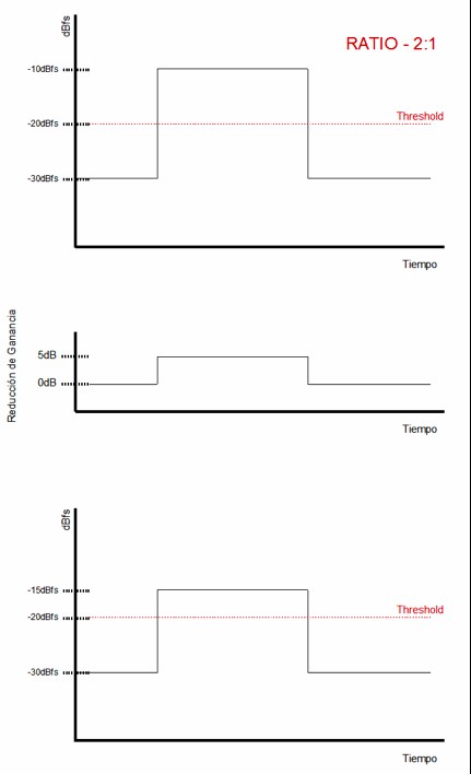
Let’s examine some examples. To simplify things, imagine we are working in the digital domain, where levels are expressed in dBFS: 0 dBFS is the maximum level, and all other values are negative. Imagine we insert a compressor on a track, set the threshold to –20 dBFS, and choose a 2:1 ratio. Now imagine that at a certain moment, the incoming signal reaches –10 dBFS. The portion that exceeds the threshold is the range between –20 dBFS and –10 dBFS—that is, a difference of 10 dB. With a 2:1 ratio, only 5 dB of that excess will remain at the output, meaning the output level will be –15 dBFS. We have gone from –20 dBFS to –15 dBFS, resulting in 5 dB of gain reduction. Now imagine that under the same conditions we use a 4:1 ratio. The 10 dB that exceed the threshold will be reduced so that only 2.5 dB remain above it. The output level would then be –12.5 dBFS. As we can see, increasing the ratio produces more gain reduction—we go from 5 dB of reduction to 7.5 dB.

Let’s now look at what happens if we place the threshold lower in relation to the signal. Imagine we set the threshold at –40 dBFS with a ratio of 2:1. Since the peak reaches –10 dBFS, we are exceeding the threshold by 30 dB. This means that at the output, we would exceed the threshold by 15 dB, giving us an output level of –25 dBFS. Therefore, with a 2:1 ratio, placing the threshold at –20 dBFS results in an output level of –15 dBFS, while placing the threshold at –40 dBFS results in an output of –25 dBFS.

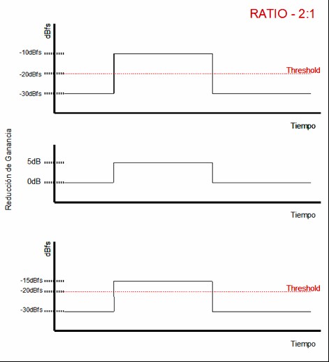
Compression with a 2:1 ratio and a –20 dBFS threshold on a signal peaking at –10 dBFS

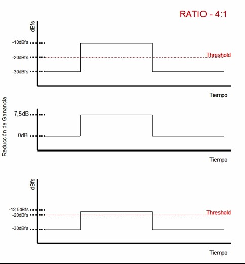
Compression with a 4:1 ratio and a –20 dBFS threshold on a signal peaking at –10 dBFS

From all of this, we can draw two important conclusions:

• Lowering the threshold results in more gain reduction.
• Lowering the ratio results in less gain reduction.

Let’s now move on to the time constants. Attack time is the amount of time it takes for the compressor to reach full gain reduction, while release time is the amount of time it takes for the compressor to return from maximum gain reduction back to unity gain.

Let’s illustrate this with an example. Imagine we have a signal at a steady level of –30 dBFS. At a given moment, the level suddenly jumps to –10 dBFS, and after a brief period, it drops back to –30 dBFS. Imagine we insert a compressor on this track, set the threshold to –20 dBFS, and choose a ratio of 2:1. Let’s also assume we set the attack time to 2 ms and the release time to 2 ms. Before considering the time constants, let’s analyze the situation exactly as we have been doing so far. We have 10 dB of signal exceeding the threshold, and with a 2:1 ratio, we will get 5 dB of gain reduction. Therefore, when the signal reaches –10 dBFS, the compressor output will be –15 dBFS.

Compression with attack and release times set to 0 seconds

Now let’s see what happens when we introduce time constants into the analysis. Initially, both the input and output levels are at –30 dBFS. At a certain moment, the input signal jumps instantly to –10 dBFS. At that moment, the compressor begins applying gain reduction gradually until reaching the full 10 dB of reduction, which takes 2 ms. This means that at the output, we initially get –10 dBFS, and after 2 ms we reach –15 dBFS. After those 2 ms, the output remains attenuated by 10 dB until the input signal drops back down to –30 dBFS. At that moment, the output level becomes –35 dBFS, because the compressor does not return to unity gain instantly—due to the release time we have set, gain reduction continues momentarily. Gradually, the output returns to –30 dBFS, taking exactly 2 ms to do so.

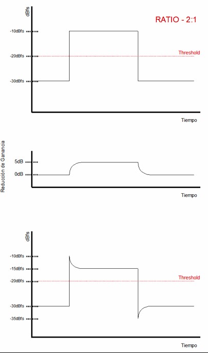
Same compression as in the previous figure, but with attack and release times different from 0s

Later on we will look at practical considerations regarding how to configure time constants. For now, it’s important simply to understand what they are and how they affect the signal.

Transfer Functions

At this point, it would be useful to understand what transfer functions are. When working with dynamic processors, it is very common to come across these kinds of graphs, especially in manuals and in the graphical interfaces of many compressor plugins. You will see how these graphs make it very easy to calculate everything we’ve been discussing so far, but I preferred not to introduce them earlier so that you could first understand how threshold and ratio behave through traditional calculations.

A transfer function is a graph that compares input level against output level, allowing us to determine what output level we will get for any given input level.

Let’s begin by looking at a unity-gain function:

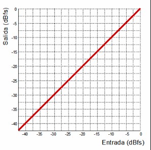
Unity-gain transfer function

This could represent the transfer function of any processor set to bypass. To interpret these graphs, we look at the input value and then see where the corresponding output falls. For example, if we look at an input level of –10 dBFS and follow where it intersects the red line, we see that the output is also –10 dBFS.

Now let's look at the transfer function of an amplifier:

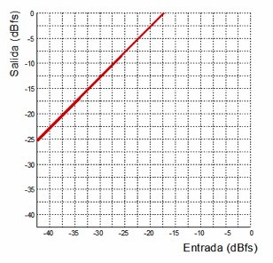
Transfer function of an amplifier with a gain factor of 2.4

This transfer function can be interpreted as the behavior of a linear amplifier—that is, the output is the input multiplied by a fixed value. For example, if we look at an input of –30 dBFS, the output would be –12.5 dBFS. We can see that for any input value, the output corresponds to the input multiplied by 0.41. Keep in mind that we are working in dBFS, which is a negative scale. In reality, that 0.41 factor indicates that we are applying a gain of 2.4 times the input signal.

Here is the inverse curve:

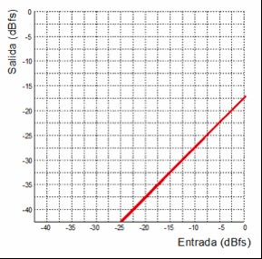
Transfer function of an attenuator with an attenuation factor of 2.4

In this case, we have the transfer function of an attenuator that operates with the same factor as the amplifier example.

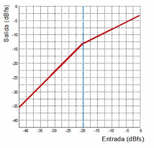
Now let’s look at the transfer function of a compressor:

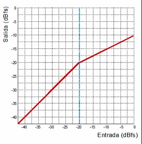
Compressor transfer function with a threshold at –20 dBFS and a ratio of 2:1

The compressor described by this transfer function is the same one we examined earlier when discussing ratio. We see that the signal is at unity gain up to –20 dBFS. From that point onward, the output no longer matches the input; instead, it is reduced to half the level of anything exceeding the threshold. This corresponds to a compressor with a threshold at –20 dBFS and a 2:1 ratio. By looking at this simple graph, we can immediately determine everything we previously calculated manually. For example: What is the output for an input of –10 dBFS? How much gain reduction is applied? According to the graph, an input of –10 dBFS gives an output of –15 dBFS, meaning we have 5 dB of gain reduction, since the expected unity-gain output would have been –10 dBFS.

We can see that transfer-function graphs are a very convenient way to visualize how a device behaves, without needing to do any math or strain our brains.

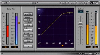
Example of a compressor plugin where we can see the transfer function (Waves C1)

Other Controls in a Compressor

Aside from the basic controls we’ve already discussed, many compressors offer additional parameters that allow us to further tailor the device depending on the purpose of the compression. The most notable ones are the following:

Some compressors give us the ability to control how the device transitions from unity gain into compression—that is, how it moves from a ratio of 1:1 to the ratio we’ve set. The two most common options are hard-knee and soft-knee.

All the examples we’ve explored so far have referred to a hard-knee configuration, where the selected ratio is applied immediately once the signal exceeds the threshold. In soft-knee mode, the transition from unity gain to the selected ratio occurs gradually along a curve, meaning the ratio increases progressively from 1:1. It’s important to understand that this curve affects both sides of the threshold, which has two consequences. First, compression begins slightly below the threshold (at its mildest values during the gradual ratio increase). Second, the selected ratio is not reached immediately above the threshold. Therefore, the applied ratio depends on the input level—the higher the signal, the closer it gets to the selected ratio.

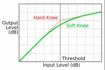
Transfer function with hard-knee and soft-knee

Additionally, some compressors allow the slope of the knee to be modified gradually—for instance, Sonnox Dynamics provides four different knee settings.

Different knee configurations in Sonnox Dynamics

As you can imagine, hard-knee mode results in much less subtle compression compared to soft-knee. Therefore, we choose soft-knee when we want the compression to be as transparent as possible and not easily noticeable.

Most compressors also include an output gain control called make-up gain. Since compression reduces the signal level, this control allows us to compensate for the lost gain. It’s very important to remember that this gain applies to the entire output signal—both the unprocessed part (below threshold) and the processed part (above threshold). I usually adjust the make-up gain so that the processed signal has the same loudness as the unprocessed one, allowing me to make meaningful A/B comparisons and clearly hear what the compressor is doing.

Compressor transfer function with a threshold at –20 dBFS, a 2:1 ratio, and 7.5 dB of make-up gain

Another very useful feature offered by many compressors is the ability to apply filtering to the key signal. This works exactly like the key-filter options available in gates and expanders that we discussed in the previous chapter, so we won’t repeat that explanation here.

Some compressors may include other additional controls, may use different names for the same controls, or may omit some of these parameters entirely. The best approach, once the fundamentals are understood, is to skim through the manuals of the devices you use to understand their specific characteristics.

Parallel Compression

So far, we have seen how compression affects the transients of our signals, since it reduces the output level during the loudest portions of the audio. However, sometimes we want to compress a signal while preserving its original transients exactly as they appear at the input. To achieve this, we use what is known as parallel compression, or New York-style compression (named after the engineers in that city who first adopted this technique).

Parallel compression consists of duplicating the signal we want to compress, applying compression to that duplicate, and then blending the compressed signal with the original. We can do this easily by duplicating the track—including all its inserts. However, this approach has two disadvantages. First, duplicating all the insert effects unnecessarily increases CPU load. Second, if we make any changes to the original track, we must replicate those changes in the duplicated track. The most common and efficient way to set up parallel compression is the same method used in analog mixing. We send the original signal to an auxiliary bus so that any change in the original automatically affects what is sent to the bus. Under normal circumstances, this send should be at unity gain (we must send the exact same level as the audio track). We then create a track whose input is that auxiliary bus, insert a compressor on it, and configure it for heavy compression (at least 8 dB of gain reduction in typical situations) with the fastest attack possible. Once the compressor is set, we pull the fader of the compressed track all the way down and slowly bring it up, blending the compressed signal with the original.

This approach allows us to compress the signal while preserving its original transients, because instead of reducing the peaks (as in normal compression), we are effectively raising the low-level content. This results in much less aggressive compression compared to traditional downward compression.

I tend to use this technique exactly as described when I need very transparent compression. For example, in a jazz album we might have a vocal with too wide a dynamic range, but using normal compression could destroy the natural character required for this genre. Applying parallel compression allows us to control dynamics while maintaining the natural tone.

I also use parallel compression when I want to add body to a drum kit. Normally, I follow the same approach described above, except that instead of sending only one signal, I send all drum tracks to the parallel compression bus. This allows the whole kit to be compressed while maintaining the transient definition that we have shaped with compressors on each individual drum track. However, sometimes we can creatively adjust the send levels to make individual elements more prominent in the mix. For example, if we feel the snare is not defined enough, increasing its send level to the parallel compressor can make it stand out more clearly with just a small adjustment.

Until now, we’ve viewed parallel compression as a static uncompressed track blended with a heavily compressed version of the same signal—bringing up the fader of the compressed track from the bottom until we find the desired balance. However, there are situations where we may need to do the exact opposite. Imagine we have a song in which we want a very dense drum sound. To achieve this, it’s common to apply standard compression to a drum subgroup. In this case, instead of using sends, we route the outputs of the drum tracks directly to the input of the subgroup. The compressed drum bus may give us a sound we like, but we might also notice that we’ve lost much of the transient character we previously shaped on each individual track before the bus compression. To solve this, we can send the specific elements that lost their transient character—via sends—to a new track, and gradually raise that fader until we recover the desired attack.

Where Should Things Go?

Many people wonder where to place the compressor—before or after the equalizer? To answer this, we must keep in mind that compression alters the frequency balance of the signal, and that low frequencies tend to trigger a compressor more strongly than high frequencies. Given these two facts, we can assume the following: if the compressor is placed before the EQ, the frequencies we intend to remove will still influence the compression; if the EQ is placed before the compressor, the compression will alter the tonal balance we just shaped with the EQ.

To avoid this problem, I usually apply EQ in two stages. In the first stage, I use a transparent equalizer to apply a high-pass filter and remove unwanted resonances. Once the signal is cleaned up, I insert the compressor and set the dynamics. After compression, I place another EQ to establish the final tonal balance.

If we do it this way, the EQ responsible for shaping the frequency balance will not be influenced by compression. If we did not follow this approach, any EQ adjustment would alter the compression behavior, meaning we’d constantly have to readjust both the EQ and the compressor.

In addition to EQ in two stages, I also often use two stages of compression when needed. Classic compressors (1176, LA-2A, 660, etc.) impart a certain character to the sound, and we won’t always use them strictly for dynamic control. We can first manage the dynamics with a VCA compressor, and then insert one of these character compressors afterward if we want a special tone. We can also distribute different dynamic tasks across multiple compressors, making the workflow more efficient. For example, on a snare we might want to both level the signal and add punch. We can use one compressor for leveling and another to enhance attack. When doing this, we must ensure the time constants of each compressor do not interfere with each other.

It’s important to remember that there is no universal rule dictating the order of EQs and compressors. We should arrange them in whatever way best suits each situation. And we should never be afraid to insert as many compressors or equalizers as we feel necessary. When mixing, we must be free to break rules to achieve the result we want.

Mix Bus Compression

The use of a compressor on the mix bus is something that has been done for a very long time, and for just as long it has remained a topic of debate among audio engineers. First of all, it’s important to note that there are excellent mix engineers who mix through a bus compressor, and many other excellent engineers who prefer not to. Therefore, using or not using a mix bus compressor is not what determines whether a mix is good—it ultimately comes down to personal preference.

Many people believe that using a compressor on the mix bus means encroaching on the mastering engineer’s job. However, this is not the case. Inserting a compressor on the master channel once the mix is finished—or close to being finished—makes no sense, because doing so alters the balance we worked so hard to achieve during the mix. In that situation, yes, we would be stepping into the mastering engineer’s territory, and the compressor would not provide any real benefit to the mix itself. Using a compressor on the mix bus means mixing through that compressor from the very beginning. This way, all our decisions and adjustments during the mix are influenced by the compressor’s behavior, and therefore the compressor becomes an essential part of the mix process.

If you’re new to mixing, I recommend avoiding mix bus compression until you fully understand compressors and how they affect audio. A poorly set mix bus compressor can force you to scrap the entire mix.

When I mix through a compressor, I find several advantages. First, it allows me to achieve the overall dynamic balance of the mix while applying much less compression on individual tracks. I especially notice this when working on level balancing. The mix starts to feel cohesive much more quickly—elements seem to “glue” together faster than when relying solely on individual compression. Additionally, mixes done through a bus compressor typically require fewer automations. This is because the compressor naturally shapes the relative levels between elements, reducing the need for complex automation moves.

However, mixing through a compressor also means that some things we previously assumed to be true no longer behave the same way. For instance, since all elements are being compressed together, fader movements no longer produce the same results. Imagine (or try it) compressing a bus containing all drum elements and then slowly raising the snare fader. You’ll notice that the change affects not only the snare’s level but also the rest of the kit and the perceived punch of the drums. The same thing happens when mixing through a mix bus compressor. Achieving good results requires some experience.

When using a mix bus compressor, it’s crucial to keep gain reduction very low. Often, just 1 or 2 dB is enough. In special cases you might go up to 4 dB, but I personally limit myself to 2 or 3 dB in the loudest sections of the song. Attack and release times are also extremely important, as they determine whether the compressor introduces unwanted artifacts. For example, an attack time that’s too fast will completely remove the mix’s transient character, making it sound lifeless, dark, and flat. I generally use an attack time between 3 and 4 ms and a release time between 200 and 300 ms. These settings must be adjusted according to the tempo of the song. The ratio used on mix bus compressors is typically very low—around 1.5:1 or 2:1.

As always, the best thing to do is simply experiment. Try mixing a track with a compressor on the mix bus—you may love the result, or you may hate it. As we’ve said, it all comes down to personal taste.

This concludes this installment. Unfortunately, we’ve had to cover quite a bit of theory which, although sometimes tedious, is essential. As compensation, in the next installment we’ll have very little text and lots of practical examples in the form of audio and video, where you’ll be able to hear for yourself what dynamic processors can do and explore some advanced dynamic-processing techniques. Until then… a warm hug.

Author: José A. Medina (2013)